2.24
2025-02-24
核密度估计
通过 一个知乎回答 学习了核密度估计(Kernel density estimation,KDE),能够用样本估计概率密度函数。
可以通过一个简单的 python 程序展示 KDE 的效果(使用高斯核函数):
import matplotlib.pyplot as plt
import numpy as np
import scipy.stats as stats

dataAmount = 10 ** 5
xAmount = 10 ** 4
data = np.random.uniform(-10, 10, dataAmount)
x = np.linspace(-10, 10, xAmount)
kde = stats.gaussian_kde(data)
density = kde(x)

plt.plot(x, density)
plt.show()
输出如下:
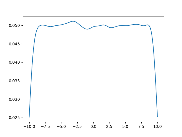 极限的理想情况是在中间呈现均匀分布,但
 dataAmount 和 xAmount 都有限,我们希望在相同计算量的情况下达到最好的效果。
计算量
对于计算量,从 KDE 公式上看,复杂度应该是 dataAmount * xAmount ,但测试发现并非如此:
startTime = time.perf_counter()

def startCount():
    global startTime
    startTime = time.perf_counter()

def printTime(x:str):
    global startTime
    print(x + ": " + (time.perf_counter() - startTime).__str__())
    startTime = time.perf_counter()

for i in range(5, 9):
    j = 9 - i
    dataAmount = 10 ** i
    xAmount = 10 ** j
    data = np.random.uniform(-10, 10, dataAmount)
    x = np.linspace(-10, 10, xAmount)
    startCount()
    kde = stats.gaussian_kde(data)
    kde(x)
    printTime("data amount = {}, xAmount = {}".format(dataAmount, xAmount))
输出:
data amount = 100000, xAmount = 10000: 5.868209599982947
data amount = 1000000, xAmount = 1000: 8.375833499943838
data amount = 10000000, xAmount = 100: 12.967822499922477
data amount = 100000000, xAmount = 10: 20.36547399999108
进一步实验:
results = np.full((10, 10), np.nan)
for i in range(1, 10):
    for j in range(1, 11 - i):
        dataAmount = 10 ** i
        xAmount = 10 ** j
        data = np.random.uniform(-10, 10, dataAmount)
        x = np.linspace(-10, 10, xAmount)
        startCount()
        kde = stats.gaussian_kde(data)
        kde(x)
        results[i][j] = time.perf_counter() - startTime

df = pd.DataFrame(results)
df.drop(columns=[0], index=[0], inplace=True)
print(df.to_string(na_rep=''))
输出:
| 1 | 2 | 3 | 4 | 5 | 6 | 7 | 8 | 9 | |
|---|---|---|---|---|---|---|---|---|---|
| 1 | 0.032673 | 0.000223 | 0.00274 | 0.001742 | 0.006912 | 0.063041 | 0.632997 | 6.311374 | 78.66403 |
| 2 | 0.021071 | 0.000292 | 0.003947 | 0.006638 | 0.068121 | 0.605103 | 5.983759 | 60.18651 | |
| 3 | 0.000999 | 0.001523 | 0.006448 | 0.060406 | 0.584952 | 5.902063 | 58.92799 | ||
| 4 | 0.003021 | 0.006319 | 0.057359 | 0.577309 | 5.777679 | 58.72213 | |||
| 5 | 0.008281 | 0.064728 | 0.584895 | 5.897568 | 59.1081 | ||||
| 6 | 0.124268 | 0.879937 | 8.686681 | 84.32257 | |||||
| 7 | 1.678993 | 12.47852 | 123.3277 | ||||||
| 8 | 19.62004 | 156.6667 | |||||||
| 9 | 361.3757 |
可以看出,dataAmount 相比关于 XAmount 的增长实际上更快
视觉效果
def generate_kde(i, j):
    dataAmount = 10 ** i
    xAmount = 10 ** j
    data = np.random.uniform(-10, 10, dataAmount)
    x = np.linspace(-10, 10, xAmount)
    kde = stats.gaussian_kde(data)
    return (x, kde(x))

rows, cols = 8, 8
fig, axes = plt.subplots(rows, cols, figsize=(11, 11))

for i in range(rows):
    for j in range(cols):
        if (i + j >= 8):
            axes[i, j].axis('off')
        else:
            ax = axes[i, j]
            ax.set_xticks([])
            ax.set_yticks([])
            x, kde = generate_kde(i + 1, j + 1)
            ax.plot(x, kde)
            ax.set_title(f'({i + 1},{j + 1})')

plt.show()
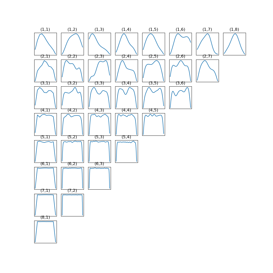 可以看出,
可以看出,dataAmount 比 XAmount 的作用大得多!
图书馆
今天翘了三节课,有些愧疚,于是晚八点来图书馆学习。明明学期刚开始,图书馆已经人满为患(虽不及期末周)

给日寄都用 Table of Contents 插件加上了静态目录,然后爽爽学概率论!
\begin{aligned}\mathcal{F}f(s) &= \int_{-\infty}^{+\infty}{f(x)\mathrm{e}^{-2\pi is}dx}\ &= \int_0^{+\infty}{\mathrm{e}^{-\beta x}\mathrm{e}^{-2\pi isx}dx}\ &= \int_0^{+\infty}{\mathrm{e}^{-(\beta+2\pi is)x}dx}\ &= \left[\frac{\mathrm{e}^{-(\beta+2\pi is)x}}{\beta+2\pi is}\right]_0^{+\infty}\ &= \frac{1}{\beta+2\pi is} \end{aligned}$$
Now, let
So
这可以用于轻松地证明《普林斯顿概率论读本》习题 15.10.22:证明柯西分布是稳定的
猫
图书馆


评论区
最新评论
--